Intro

A token buyback happens when a protocol uses non-native assets, such as stablecoins, ETH, or other liquid reserves, to repurchase its own token from the open market. 

The purpose is to align token value with economic activity by creating market demand and reducing circulating supply. 

After a buyback, tokens can follow different paths depending on the design of the system:

1. Burned: permanently destroyed to increase scarcity.

2. Retained: kept in the treasury to be used later for staking rewards, governance participation, or liquidity.

3. Recycled: distributed again through incentive programs, shifting ownership from sellers to active users.

A true buyback must use external capital. Moving tokens already held in the treasury, or locking them under a vesting schedule, doesn’t change the market structure, it doesn’t absorb supply or add buy pressure.

Value Accrual

To understand why buybacks matter, it’s necessary to first understand value accrual.

In token economics, value accrual describes the process through which a token captures part of the economic value created by the protocol. It’s the point where growth, usage, or fees generated within the system translate into value for token holders, either through price appreciation, yield, or increased purchasing power within the ecosystem.

Buybacks fit into this last category. When a protocol uses real revenue to repurchase its token, it converts operational performance into market demand. Each repurchase effectively transfers value from the protocol’s income to token holders by reducing supply and increasing each token’s proportional claim on the system’s future output.

In this sense, buybacks are one of the cleanest value-accrual mechanisms available.

To see how this works in practice, let’s look at Hyperliquid — one of the cleanest examples of a direct value accrual loop.

Example: Hyperliquid’s Buyback Loop

A clear example of value accrual through buybacks can be seen in Hyperliquid, one of the fastest-growing on-chain derivatives exchanges.

Hyperliquid charges trading fees in USDC and directs a portion of those fees toward repurchasing and burning its native token, HLP.

Each time a trade occurs, part of the protocol’s real cash flow (denominated in stable assets) is converted into demand for HLP on the open market. These tokens are then permanently destroyed. The effect is twofold: it reduces circulating supply and anchors token value to actual exchange activity.

This model creates a transparent feedback loop between protocol performance / revenue and token holder benefit.

1. When trading volume increases, more fees are generated.

2. Higher fees mean larger buybacks.

3. Larger buybacks mean fewer tokens in circulation and a stronger link between real usage and token value.

It’s a direct and measurable form of value accrual: every dollar of revenue partially flows back into the token itself.

This creates a deterministic mapping between network activity and token scarcity:

Network activity → fees → buybacks → supply contraction

From a game-theoretic perspective, Hyperliquid’s buyback model creates alignment across all participants in the system.

Traders use the product for execution quality, liquidity, and speed, not speculation. Their activity generates fees that fund the buybacks, converting product usage into token demand without forcing traders to hold the token.

Holders benefit from this flow as each buyback reduces circulating supply and increases their proportional claim on the system’s future value. The rational strategy is to hold longer, since value compounds over time through continued buybacks.

The team is aligned with holders through its token allocation, which grows in value as trading volume and revenue increase. This structure pushes them to focus on product performance and real growth rather than short-term price movements.

The protocol treasury acts as the coordinating mechanism, allocating a fixed share of revenue to buybacks and maintaining predictable rules that participants can anticipate and model.

Buyback Framework

Designing a buyback framework requires more than deciding if tokens should be repurchased. It defines how, when, and why capital flows back to the token.

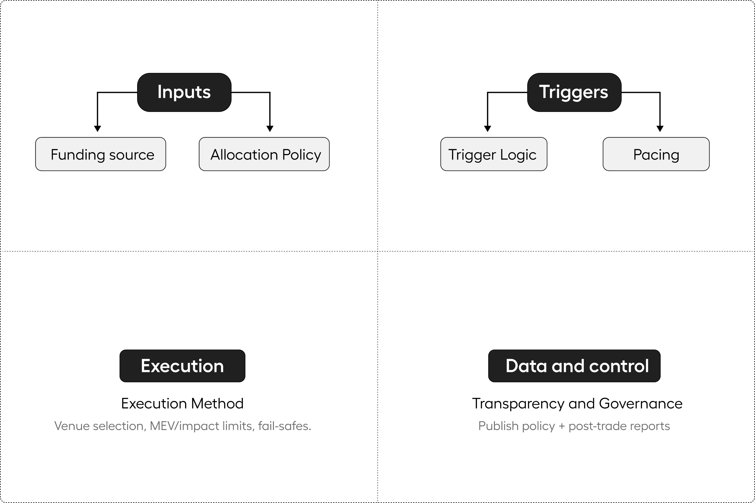
The buyback framework we designed and use has seven key components:

1. Funding Source: A buyback must use real external assets. That can include protocol revenue, stablecoin reserves, or fee income, but never the project’s own token supply.
   
   

2. Allocation Policy
   This defines what portion of earnings or treasury assets is directed toward buybacks. The optimal allocation depends on stage and cash flow stability.
   
   

3. Trigger Logic
   The trigger determines when buybacks occur.
   
   

4. Pacing and Smoothing
   Timing matters as much as direction.
   
   

5. Execution Method
   How tokens are purchased affects both cost and signaling.
   
   

6. Transparency and Governance
   Buybacks must be transparent without exposing exploitable information.
   
   

7. Objective and End State
   Finally, every buyback needs a defined purpose. Some aim to reduce float and stabilize price. Others accumulate tokens for staking rewards, liquidity, or treasury rebalancing. The end state determines whether tokens are burned, retained, or redistributed.

When these components work together, the buyback becomes a monetary policy tool.

Funding Source

The foundation of any buyback framework is the capital it draws from. A buyback must use external, productive assets, such as stablecoins, ETH, or protocol revenue, not the project’s own token supply. This distinction is critical because only external assets create genuine market demand and reduce circulating supply.

The credibility of the program depends on where this capital originates.
Buybacks funded by recurring revenue reflect a healthy, cash-flow-generating business model. They demonstrate that the protocol can reward holders without weakening its reserves.

Allocation Policy

The allocation policy defines how much of the protocol’s income or treasury capital is directed to buybacks. It is the protocol’s version of a “dividend ratio.”
The objective is to find a balance between three competing needs: growth, liquidity, and value distribution.

When revenue is volatile or early-stage, allocation should stay below 20% of net income.

Once monthly revenue variance falls under 30%, allocation can increase to 30–50%.

Protocols with long-term predictable income streams (e.g., exchanges or L2s with stable fee models) can safely commit 50 to +70%.

Best Practice: Use rolling 90-day revenue averages to adjust the allocation ratio dynamically. This creates a self-calibrating policy that scales with financial stability.

Its important to avoid setting a static allocation percentage (e.g., “30% of revenue”). Instead, define dynamic bands based on revenue performance and market conditions.

To measure efficiency objectively, many protocols use the Price-to-Sales (P/S) ratio, a metric that compares the token’s market capitalization to the protocol’s annualized revenue.

Price-to-Sales (P/S) ratio

P/S = Market Capitalization ÷ Annualized Revenue

It tells you how much investors are paying for each dollar of protocol revenue. A lower P/S implies the token is undervalued relative to its fundamentals, while a higher P/S indicates that it trades at a premium.

For example, if a project has a $500M market cap and generates $50M in annualized revenue, its P/S ratio is 10×. If revenue doubles to $100M while market cap remains constant, the P/S ratio drops to 5× — meaning the token has become cheaper relative to its economic performance.

In buyback design, this matters because a P/S-based trigger ensures capital is deployed when the market undervalues the protocol, maximizing the number of tokens repurchased per dollar spent and preserving treasury efficiency.

Static ratios ignore how efficiently each dollar spent converts into value. A smarter policy links buyback intensity to quantifiable indicators such as valuation (P/S), revenue stability, and treasury strength.

Let’s assume a protocol generates $25,000 per day in real revenue, which annualizes to $9.1 million and its token currently trades at a market capitalization of $16.87 million.

P/S = $16.87M ÷ $9.125M = 1.85×

At 1.85×, the token trades far below the industry average (typically 5×–12× for similar projects). This means the market is undervaluing each dollar of protocol revenue — a prime condition for buybacks.

Using valuation-aware allocation bands, the policy might look like this:

At 1.85×, the project sits inside the extreme value band, a prime condition for buybacks financed by real revenue.

Earnings-Based Valuation (P/E and SWPE)

While the Price-to-Sales (P/S) ratio measures how the market values revenue, it doesn’t capture how efficiently that revenue converts into actual profit. The Price-to-Earnings (P/E) ratio — and its float-adjusted variant, the Supply-Weighted P/E (SWPE) — adds that layer of precision.

The P/E ratio compares a project’s market capitalization to its net earnings, showing how much investors are paying for each dollar of profit. In traditional finance, a lower P/E suggests stronger profitability relative to price — the same applies in token economies.

However, because most tokens have large locked supplies that distort valuation metrics, a Supply-Weighted P/E (SWPE) offers a cleaner view. It adjusts for circulating supply, reflecting the real ratio between earnings and the liquid portion of the token supply.

SWPE = (Market Cap ÷ Earnings) × (Circulating Supply ÷ Total Supply)

A lower SWPE indicates stronger demand relative to circulating float, meaning each token absorbs more economic output per unit of supply. In this context, the SWPE ratio helps calibrate buybacks with higher accuracy, ensuring that capital is deployed when profitability is high, circulation is tight, and valuation remains attractive.

For example, Hyperliquid maintains a SWPE ratio in the range of 2× to 3× during peak fee periods. That suggests the market is pricing its token at roughly two to three times its protocol earnings after adjusting for float, a range often associated with undervaluation in traditional equity terms.

When integrated into buyback design, SWPE serves as a profitability trigger:

• High SWPE → earnings overpriced, preserve cash.

• Low SWPE → earnings undervalued, buy aggressively.

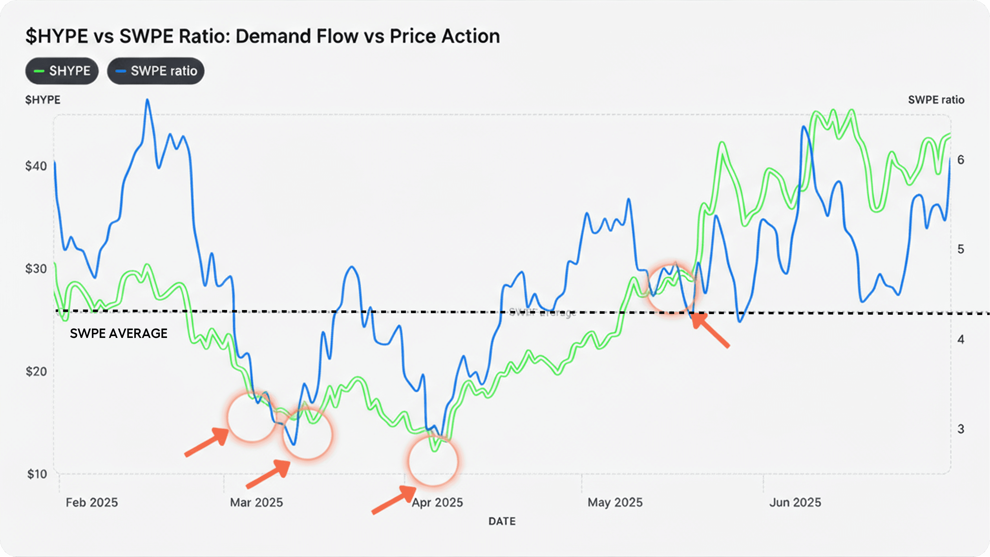
Case Study: Hyperliquid’s SWPE as a Buyback Signal

Hyperliquid offers one of the clearest real-world examples of how valuation metrics can guide buyback efficiency. The protocol allocates 97% of its earnings to repurchasing HYPE through its Assistance Fund (AF), creating sustained demand while reducing float.

The key indicator used to monitor this system is the Supply-Weighted P/E (SWPE) ratio.

Over the past year, SWPE has become one of the most reliable on-chain buyback signals for HYPE. When SWPE falls below 3.0, it has historically marked strong accumulation zones for investors and traders. When it rises above 6.0, the market tends to be overheated.

More depth on this here

While SWPE measures how efficiently a protocol converts earnings into market value, it still focuses on performance within the current circulating supply. To capture the long-term impact of future unlocks and potential dilution, the analysis must extend beyond earnings efficiency to the token’s total implied valuation.

That’s where the Dynamic FDV Buyback model comes in. It links buyback allocation to the token’s fully diluted valuation, ensuring capital is deployed most aggressively when the market undervalues the entire supply, not just the active float.

Dynamic FDV Buyback

It adjusts buyback intensity not just to market capitalization but to the total implied valuation (FDV) of the token. The framework links buyback allocation inversely to valuation, ensuring capital efficiency and treasury discipline. Example:

This ensures that buybacks are most aggressive when the token’s fully diluted value is low (maximizing tokens repurchased per dollar) and taper off as valuation expands.

If applied in isolation, a Dynamic FDV Buyback model can introduce several structural weaknesses that undermine its intended stabilizing effects.

When the mechanism relies solely on fully diluted valuation bands without integrating liquidity, revenue stability, or unlock schedules, it risks becoming reactive rather than strategic. FDV, by nature, is a forward-looking metric inflated by unvested or illiquid supply. It can remain high even when circulating liquidity is weak, leading to reduced buyback intensity precisely when the token most needs market support.

While valuation-based frameworks like P/S and FDV models focus on fundamentals, some protocols prefer technical triggers that react purely to market behavior.

Which Framework Works Best?

Each model captures a different part of the picture. The P/S ratio shows how the market values a project’s revenue, SWPE measures how efficiently those earnings translate into profit, and FDV highlights future dilution and supply pressure. None of them tells the full story on their own, but together they can give a balanced view.

Trigger Logic

Once valuation inputs like P/S, FCF Yield, and FDV are established, the next layer defines when buybacks should actually occur. Trigger logic transforms valuation data into actionable policy. It’s the mechanism that decides if capital should enter the market today, tomorrow, or wait for better conditions.

Multi-Layer Trigger Design

Effective buyback programs often combine fundamental, liquidity, and structural triggers.

• Fundamental triggers (like P/S or FDV) define the economic threshold for undervaluation.

• Liquidity triggers ensure that daily buyback size never exceeds a certain percentage of circulating trading volume (e.g., ≤3–5%), preventing slippage and market impact.

• Structural triggers ensure the treasury or revenue pool maintains minimum reserves before capital is deployed, protecting long-term sustainability.

Trigger Hierarchy Example

• Primary Trigger: Valuation band (e.g., P/S < 4× or FDV < $50M)

• Secondary Trigger: Liquidity condition (≥ 3× daily buyback coverage)

• Safety Trigger: Treasury or runway ratio (≥ 12 months of expenses)

By sequencing triggers this way, protocols prevent reflexive or sentiment-driven execution. Buybacks activate when undervaluation coincides with sufficient liquidity and balance-sheet resilience.

Trigger Calibration
Even with predefined thresholds, triggers should evolve as the protocol matures. Early-stage projects may rely more on valuation triggers (since volatility is high and liquidity shallow), while later-stage protocols can integrate volume-weighted or even behavioral signals, such as deviations from long-term median price or on-chain activity flows.

Pacing and Smoothing

Once buybacks are triggered, the next challenge is pacing, which determines how fast and how often tokens should be repurchased.

Even with sound valuation logic, poor pacing can create market distortions. Deploying too quickly concentrates buy pressure into short timeframes, pushing prices up temporarily and eroding efficiency. Deploying too slowly, on the other hand, weakens the feedback loop between real revenue and market perception.

A robust pacing policy smooths buyback activity over time, aligning it with both liquidity depth and the protocol’s revenue frequency. The most common structures are daily rollovers or 30-day smoothing windows, where revenue earmarked for buybacks is averaged across a fixed period rather than spent at once.

Across the market, pacing frameworks fall into three archetypes:

Continuous (Real-Time):
Protocols such as Hyperliquid, GRAIL, and CAKE execute micro-buybacks on every transaction, creating constant on-chain demand that mirrors product activity.
This approach maximizes transparency and immediate value accrual but sacrifices capital efficiency. During volume spikes, these systems tend to overspend at market peaks, amplifying reflexivity and volatility. It works best for high-frequency environments where simplicity and correlation to real usage matter more than optimization.

Epochic (Daily or Weekly):
Projects like GMX, WOO, and JUP batch revenue over 24-hour or 7-day cycles and deploy it gradually into the market—often using time-weighted or volume-weighted averaging (TWAP/VWAP).

This pacing model smooths buy pressure, avoids overreaction to intraday volatility, and enables dynamic calibration based on valuation metrics such as FDV or P/S.
Empirically, this structure delivers the best balance between capital efficiency, signaling strength, and stability. It also allows protocols to DCA into downturns, preserving liquidity while maintaining a consistent presence in the market.

Discretionary or Quarterly:
Used by larger DAOs such as AAVE and BIFI, this model accumulates fees continuously but executes buybacks manually, usually through governance approval.
While it maximizes flexibility and allows teams to target undervaluation windows, it introduces execution uncertainty and weakens the predictability that investors rely on for modeling yield. In most cases, this structure functions more as a treasury management tool than a monetary policy mechanism.

Execution Method

Once pacing defines the temporal structure of buybacks, execution determines their actual market impact. The method used to purchase tokens influences both the cost basis and the signaling effect

Broadly, buyback execution can be categorized into three layers of increasing sophistication:

Taker-Based Execution
Most early-stage protocols start with taker orders, in other words direct market buys on spot exchanges.

While simple to automate, taker orders remove liquidity from the order book, which can create short-term price spikes followed by sharp reversals once the buying stops. This reflexivity often causes treasury inefficiency, as a significant portion of buyback capital goes into temporary price dislocation rather than long-term supply contraction.

Projects that rely exclusively on taker orders (e.g., early RAY or CAKE implementations) often experience visible price distortions around execution windows, making the buyback pattern predictable and vulnerable to frontrunning.

Maker-Based Execution
A more advanced model — used by projects such as WOO and Hyperliquid — utilizes maker orders calibrated to organic volume.

Instead of removing liquidity, the protocol provides it, allowing buybacks to blend seamlessly into market flow. Maker-based execution benefits from two effects:

1. It captures the spread rather than paying it, improving capital efficiency.

2. It reduces volatility, since buy pressure is distributed symmetrically through resting bids that adjust dynamically with trading activity. In practice, buybacks pegged to a percentage of organic volume (e.g., 2–5%) help ensure consistent support without disrupting price discovery.

Options-Based Execution (avoid this)
Some teams experiment with options-based buybacks, believing them to be a more sophisticated or capital-efficient approach. In this structure, the protocol sells cash-secured put options on its own token at predefined strike prices — for example, committing to buy its token at $0.40, $0.30, or $0.20.

In theory, this allows the project to earn a premium upfront while only purchasing tokens if the market drops to those levels. In practice, however, the benefit almost always accrues to the market maker, not the protocol.

When a project sells puts, the counterparty receives the premium immediately while assuming limited risk. If the price stays above the strike, the market maker keeps the premium and no tokens are repurchased, meaning the project’s buyback program produces no actual accumulation.

If the price falls below the strike, the project is forced to buy at that level, even if the decline continues. The result is an asymmetric exposure: the project bears the downside while the counterparty captures risk-free upside.

This model creates three structural problems:

1. Capital Inefficiency: The treasury must fully collateralize the options with stablecoins, locking capital that could otherwise be deployed in productive use or direct buybacks.

2. Yield Extraction: The market maker earns consistent yield regardless of outcome, while the project either buys high or gets nothing.

3. Asymmetric Risk: If the token keeps falling, the project continues to accumulate depreciating assets with no hedge or recovery mechanism.

In other words, this structure effectively transforms buybacks into a subsidized options desk for the counterparty.

Organic Volume

 A critical consideration in buyback execution is understanding the difference between total and organic trading volume, the share of activity driven by genuine market participants rather than short-term or artificial flows.

If a protocol executes $500,000 in daily buybacks while real organic volume is only $2.5 million, even if reported volume shows $10 million due to wash trading or internal matching, it ends up absorbing 20% of the actual liquidity. That scale is unsustainable and creates visible pressure in the market.

To stay efficient, buybacks should align with genuine liquidity depth, typically around 2 to 5 percent of organic volume per day. This allows the market to absorb buybacks naturally without creating reflexive price moves.

Understanding volume distribution also matters. Executing near areas of high trading activity, known as value zones, increases efficiency, while buying in thin liquidity areas can trigger unnecessary volatility.

The goal is simple: blend into market flow rather than disrupt it.

Transparency and Governance

A buyback framework is only as credible as its transparency. The market must be able to verify when, how, and why buybacks occur without exposing the protocol to exploitation.

The most effective approach is to publish clear rules and data, not execution details. Teams should disclose the allocation logic, valuation thresholds, and pacing methodology, but avoid revealing specific timing or order details that traders could front-run.

Buybacks can be executed through multi-signature treasury wallets or smart contracts that automate allocations based on predefined metrics such as P/S or FDV bands. This ensures governance oversight while keeping execution neutral and predictable.

Periodic reporting, such as monthly summaries of revenue used, tokens repurchased, and remaining reserves, reinforces accountability. The objective is to make the system auditable without turning it into a trading signal.

In mature protocols, governance can gradually expand to include community oversight over allocation bands, treasury management, and repurchase frequency. However, discretion should remain with the treasury team or a trusted council to preserve execution efficiency and avoid reactionary governance decisions driven by market noise.

True transparency is not about publishing every transaction; it is about building confidence that buybacks follow consistent, rules-based logic tied to real performance.

Objective and End State

Every buyback program must have a clear purpose and an endpoint. The objective defines why tokens are repurchased, while the end state determines what happens to them afterward. Without this clarity, buybacks risk becoming symbolic rather than strategic.

In early stages, the main objective is usually float reduction. Repurchasing tokens decreases circulating supply, improves price stability, and strengthens the link between protocol performance and token value. As the system matures, the objective often shifts from value concentration to value deployment — using accumulated strength to reinforce liquidity, staking, or ecosystem incentives.

The end state defines how repurchased tokens are treated.

• Burning permanently increases scarcity and is best suited for deflationary models focused on price stability.

• Treasury retention converts buybacks into balance sheet growth, allowing the protocol to use those tokens later as collateral or for liquidity provision.

• Redistribution channels tokens back into the ecosystem, rewarding active participants and reinforcing long-term alignment.

Hyperliquid and similar protocols demonstrate that buybacks can be fully self-sustaining mechanisms of value accrual.

If a token hasclear value accrual mechanism→ fees redistribution, buybacks, share of protocol earnings (via vote escrow's) then the token could reflect real economic exposure. If there aren't... well the token could still trade quite well (like UniSwap with no accrual), but the value would be speculative and not driven by fundamentals.

AGC.